Identifiability Theory

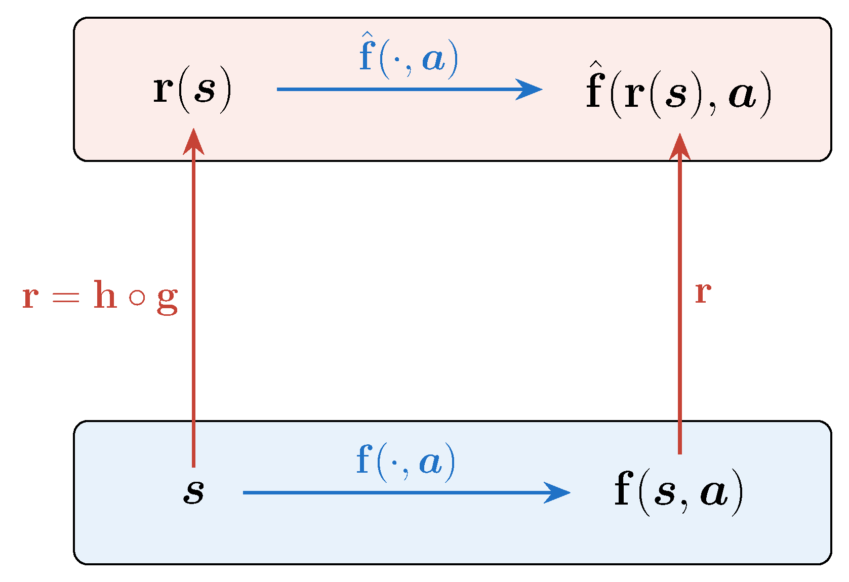
A world model is faithful when encoding and predicting commute

Let f be the true dynamics, g the observation map and h the encoder, so that states map to latents through r = h ∘ g. A learned world model is faithful if r is injective and its latent dynamics reproduce the true dynamics in latent space.

\begin{gathered}\hat{\mathbf f}\big(\mathbf r(\boldsymbol s),\,\boldsymbol a\big) \;=\; \mathbf r\big(\mathbf f(\boldsymbol s,\boldsymbol a)\big)\quad \forall\, \boldsymbol s, \boldsymbol a\\[2pt] \mathbf r = \mathbf h \circ \mathbf g\end{gathered}

This is a semiconjugacy between true and latent dynamics. It can be strengthened in steps by requiring r to be injective, a smooth diffeomorphism (nonlinear-ICA identifiability) or an affine map (linear identifiability).

We use this condition both to evaluate existing world models and to design objectives with provable recovery guarantees.

Commutative diagram: true dynamics in state space, learned dynamics in latent space, connected by r — Encoding a state after a true transition should agree with predicting from its encoded state. From Understanding the Limits of Latent World Models, Fig. 1a.

What DCL and EbC identify

Theorem 1. (Contrastive estimation of non-linear dynamics).

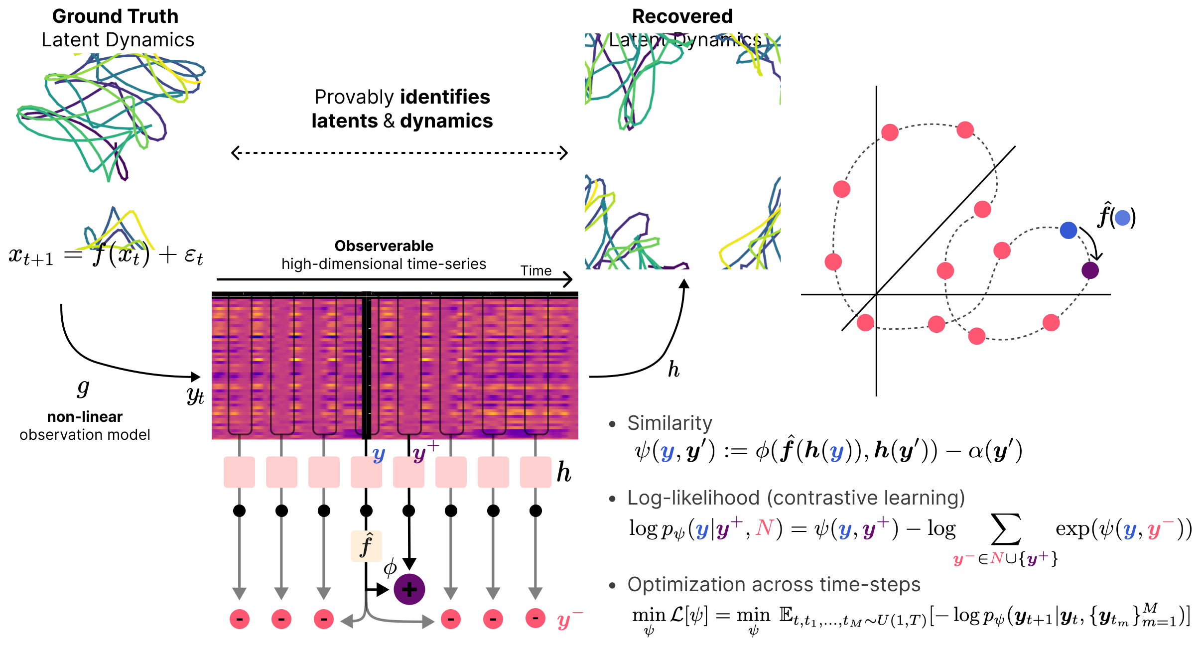
x_{t+1}=f(x_t)+\varepsilon_t,\qquad y_t=g(x_t),\qquad x_t\in\mathbb{R}^d

Assumptions.

(A1)The observed time series comes from bijective latent dynamics $f$ and an injective observation map $g$ .
(A2)System noise is independent and identically distributed: $\varepsilon_t\sim\mathcal{N}(0,\Sigma_{\varepsilon})$ , with invertible covariance.
(A3)The contrastive model uses an encoder $h$ into $d$ dimensions, a learned dynamics model, negative squared Euclidean similarity and the marginal correction $\alpha$ . It reaches the global minimum of the contrastive objective.

As the number of observations tends to infinity, the encoder recovers states by a bijective affine map on the data support, and the learned dynamics are the true dynamics expressed in those coordinates:

h(g(x))=Lx+b,\qquad L=Q\Sigma_{\varepsilon}^{-1/2},\qquad Q^\top Q=I

\widehat f(z)=L f\!\left(L^{-1}(z-b)\right)+b

$Q$ is an unknown orthogonal matrix and $b$ an offset. The marginal correction is part of the theorem, even though the paper sometimes omits it in experiments. The guarantee concerns the infinite-data optimum.

Corollary 1 · A dynamics model is necessary

Fixing the latent predictor to the identity cannot recover non-identity dynamics under the theorem’s affine identification relation. The identity system is the trivial exception.

\begin{aligned}\widehat f&=r\circ f\circ r^{-1},\qquad r(x)=Lx+b,\\\widehat f&=\mathrm{id}\quad\Longrightarrow\quad f=\mathrm{id}.\end{aligned}

Corollary 2 · Linear dynamics

For a linear system and a linear latent predictor, the state recovery remains affine and the dynamics matrices are related by a change of basis.

\begin{aligned}f(x)&=Ax,&\widehat f(z)&=\widehat A z\\\Longrightarrow\quad h(g(x))&=Lx+b,&\widehat A&=LAL^{-1}.\end{aligned}

Theorem 1. (Recovery of latents and group actions).

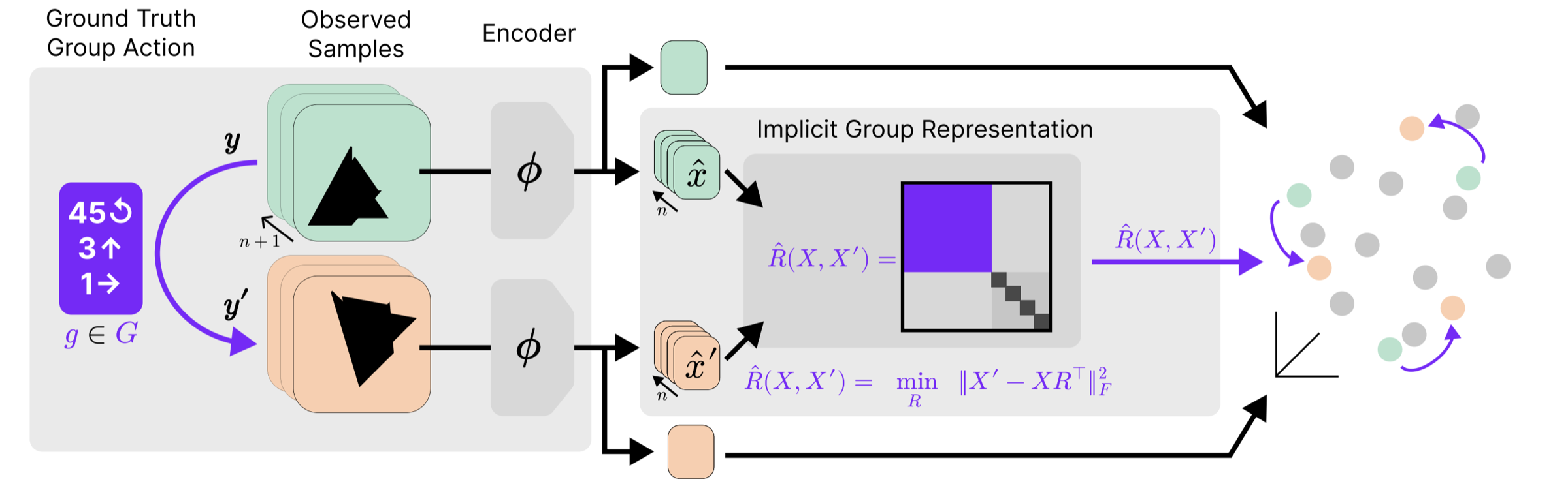
\begin{gathered}y_i=f(x_i),\quad y_i'=f(R(g)x_i),\\h=\phi\circ f,\quad R:G\to\mathrm{GL}(d).\end{gathered}

Assumptions.

(1)Injective mixing $f$ ; batches share an action $g$ . Full-rank latent sample matrices with $M>d$ allow the implicit estimator to recover $R(g)$ .
(2)Appendix A, Definition 2: candidate-feature differences span $d$ dimensions; reference-feature differences also span $d$ dimensions for each shared candidate.
(3)The learned and true-inverse conditional distributions agree: $p_{\phi}=p_{f^{-1}}$ .

On the dataset support, the paper establishes:

h(x)=Lx,\qquad L\in\mathrm{GL}(d)

R'(g):=\widehat R\big(h(X),h(gX)\big)=L R(g)L^{-1}

Here $f$ is the observation map; $g$ is a group element.

Corollary 1 · Equivariance

Encoding commutes with the group action:

h\big(R(g)x\big)=R'(g)h(x)

Theorem 2 · Appendix A.1. (Generalized canonical discriminative form).

\begin{gathered}p(y\mid x,S)=\frac{\exp\!\big(u(x)^\top v(y)+\alpha(x)+\beta(y)\big)}{\sum_{y'\in S}\exp\!\big(u(x)^\top v(y')+\alpha(x)+\beta(y')\big)},\\y\in S.\end{gathered}

Assumptions.

(1)Both models satisfy Definition 2's diversity conditions above. The vector functions $u,v$ and scalar potentials $\alpha,\beta$ may share parameters.

Matching conditionals identify both feature maps affinely on the data support:

\begin{gathered}p'=p^*\quad\Longrightarrow\quad\begin{cases}u'(x)=A u^*(x)+c,\\v'(y)=B v^*(y)+d_0,\end{cases}\\A,B\in\mathrm{GL}(d).\end{gathered}

The offset $d_0$ denotes the paper's vector $d$ .

Methods

Both are contrastive learning methods with identifiability proofs. DCL learns dynamics from time series, and EbC learns group actions from paired observations.

DCL overview: ground-truth latent dynamics, a non-linear observation model, and the recovered latent dynamics

DCLDynamics contrastive learning

ICLR 2025

DCL shows that self-supervised contrastive learning performs non-linear system identification. It uncovers linear, switching linear and non-linear dynamics under a non-linear observation model, with theoretical guarantees that latents and dynamics are recovered up to an affine map.

Self-supervised contrastive learning performs non-linear system identification
Rodrigo González Laiz*, Tobias Schmidt*, Steffen Schneider

PDF Project site arXiv OpenReview Code

EbC overview: paired observations related by a group action, an encoder, and an implicit group representation

EbCEquivariance by contrast

NeurIPS 2025

EbC learns equivariant embeddings from observation pairs related by an unknown group action. It jointly learns a latent space and a group representation in which group actions become invertible linear maps, without group-specific inductive biases, and comes with a proof of identifiability.

Equivariance by Contrast: Identifiable Equivariant Embeddings from Unlabeled Finite Group Actions
Tobias Schmidt, Steffen Schneider*, Matthias Bethge*

PDF Project site arXiv OpenReview Code